Equations for double helix in parametric form

[skr3178]

Hi,
I am working on a double helix problem for which I would like determine the equation.
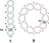
I have been able to find a few hints on other forums (Double helix)but they aren't in parametric form. In am specifically looking to determine the equation similar to picture as shown on the right of the precatenanes image.

I would appreciate any help on this.
Thanks so much

 

[Cubist]

I have a recommendation, detailed below, but it's probably biassed because I'm a programmer !

Despite this problem having a very strong mathematical element, it's much easier to tackle it using a computer programming language. I used Octave (a Matlab-like program) to generate the image below. This is a good approach because you can:-
- create a "black box" of re-usable functionality (to generate a spiral around a path)
- define intermediate/ temporary variables within functions to make subsequent expressions easier to read
- immediately plot your results to see if you're on the right track



Your problem breaks nicely down into blocks of functionality. One important function to write is:- given a point on a path (and that point's direction/velocity vector) then return a new point that is on a spiral that "orbits" in a helix around the input path (for different "t" amounts). This function could also return a velocity vector for the new point. When this is done you could call this function a second time to create a spiral around a spiral around a path.

If you really have to, after writing a successful computer program to do this - then you could then use a CAS to back-substitute all intermediate variables so that you end up with a (truly horrendous) set of 3 expressions (x,y,and z) that are purely in terms of t.

Since this is a help-site I won't just hand out my code. But I'll give you a hint, first of all write some code that produces the first helix and plots it using "scatter3()".

 

[skr3178]

Thanks for helping me out.
You image is precisely what i would like to achieve.
I have some progress on a cylindrical helix and somewhat on a toroidal helix. However, it well refined and I need help.
My code does not work well for double helix on toroid: I want to control the radius of the smaller helix and the number of turns. I would appreciate any suggestions. I have added a link to a reference for the math behind this.
REFERENCE1
All Codes are written in MATLAB

%HELIX ON HELIX_CYLINDRICAL
clear
clc
%
syms t r R h
assume(t,'real')
assume(R,'real')
assume(h,'real')
% CYLINDRICAL HELIX
x=h*t;
y=R*cos(t);
z=R*sin(t);

% % HELIX ON TORUS
% %       VARIABLES
% R=3;% MAJOR RADIUS
% r=1;% MINOR RADIUS
% n=6;% No. of loops
% x = (R + r*cos(n*t)).*cos(t);
% y = r*sin(n*t);
% z = (R + r*cos(n*t)).*sin(t);

% r_vec is the equation of the curve of interest: here helix
r_vec=[x;y;z];
dx=diff(x);
dy=diff(y);
dz=diff(z);
tan_vec=[dx;dy;dz];
nor_vec=diff(tan_vec)/simplify(norm(diff(tan_vec)));
binor_vec=simplify((cross( tan_vec, nor_vec))/norm(tan_vec));
%parametrized for the next curve
syms a
assume(a,'real')
%Number of turns of the second helix
n2=12;
u=n2*t;
S= r_vec + a.*nor_vec.*cos(u)+a.*binor_vec.*sin(u);
% VARIABLES FOR THE SECOND LEVEL HELIX
% a= radius
h_num=1; R_num=3; a_num=0.5;
S1=subs(S, [h, R, a], [h_num, R_num, a_num]);
% %%Plotting
% R=6; r=2; n=5;
t1 = 0:pi/100:40*pi;
% u1 = 0:pi/15:2*pi;
% x1=R.*cos(t)+r.*cos(t).*cos(n.*t);
% y1=R*sin(t)+r*cos(n.*t).*sin(t);
% z1=r*sin(n.*t);
% x1=S1(1)
% y1=S1(2)
% z1=S1(3)
x2=double(subs(S1(1),t ,t1)); y2=double(subs(S1(2),t ,t1)); z2=double(subs(S1(3),t ,t1));
% x3=double(subs(x2,u ,u1)); y3=double(subs(y2,u ,u1)); z3=double(subs(z2,u ,u1));

%x2=subs(x1,[t, u], [t1, u1])        
% %subs(x, t)

plot3(x2,y2,z2)
axis equal
xlabel('x(t)')
ylabel('y(t)')
zlabel('z(t)')

%   HELIX ON TORUS DIRECT FORUMLA
%
t = 0:pi/500:40*pi;
%       VARIABLES
R=3;% MAJOR RADIUS
r=1;% MINOR RADIUS
n=6;% No. of loops

xt = (R + r*cos(n*t)).*cos(t);
yt = r*sin(n*t);
zt = (R + r*cos(n*t)).*sin(t);

plot3(xt,yt,zt)
axis equal
xlabel('x(t)')
ylabel('y(t)')
zlabel('z(t)')

%
%HELIX ON HELIX_TORUS
clear
clc
%
syms t r R h
assume(t,'real')
assume(R,'real')
assume(h,'real')
% CYLINDRICAL HELIX
% x=h*t;
% y=R*cos(t);
% z=R*sin(t);

% % HELIX ON TORUS
% %       VARIABLES
R=3;% MAJOR RADIUS
r=1;% MINOR RADIUS
n=6;% No. of loops
x = (R + r*cos(n*t)).*cos(t);
y = r*sin(n*t);
z = (R + r*cos(n*t)).*sin(t);

% r_vec is the equation of the curve of interest: here helix
r_vec=[x;y;z];
dx=diff(x);
dy=diff(y);
dz=diff(z);
tan_vec=[dx;dy;dz];
nor_vec=diff(tan_vec)/simplify(norm(diff(tan_vec)));
binor_vec=simplify((cross( tan_vec, nor_vec))/norm(tan_vec));
%parametrized for the next curve
syms a
assume(a,'real')
%Number of turns of the second helix
n2=12;
u=n2*t;
S= r_vec + a.*nor_vec.*cos(u)+a.*binor_vec.*sin(u);
% VARIABLES FOR THE SECOND LEVEL HELIX
% a= radius
h_num=1; R_num=3; a_num=0.5;
S1=subs(S, [h, R, a], [h_num, R_num, a_num]);
% %%Plotting
% R=6; r=2; n=5;
t1 = 0:pi/100:40*pi;
% u1 = 0:pi/15:2*pi;
% x1=R.*cos(t)+r.*cos(t).*cos(n.*t);
% y1=R*sin(t)+r*cos(n.*t).*sin(t);
% z1=r*sin(n.*t);
% x1=S1(1)
% y1=S1(2)
% z1=S1(3)
x2=double(subs(S1(1),t ,t1)); y2=double(subs(S1(2),t ,t1)); z2=double(subs(S1(3),t ,t1));
% x3=double(subs(x2,u ,u1)); y3=double(subs(y2,u ,u1)); z3=double(subs(z2,u ,u1));

%x2=subs(x1,[t, u], [t1, u1])        
% %subs(x, t)

plot3(x2,y2,z2)
axis equal
xlabel('x(t)')
ylabel('y(t)')
zlabel('z(t)')


%%
%   HELIX ON TORUS DIRECT FORUMLA
%
t = 0:pi/500:40*pi;
%       VARIABLES
R=3;% MAJOR RADIUS
r=1;% MINOR RADIUS
n=6;% No. of loops

xt = (R + r*cos(n*t)).*cos(t);
yt = r*sin(n*t);
zt = (R + r*cos(n*t)).*sin(t);

plot3(xt,yt,zt)
axis equal
xlabel('x(t)')
ylabel('y(t)')
zlabel('z(t)')

 

[Cubist]

I've had a quick look at your code. I don't see any functions in there, but it looks like you've spent a lot of time. To obtain an "easy" result you really need to have a function that will return a helix around a previous path. I include my solution below. I hope you can follow it (I wrote it very quickly ?)...

Spoiler: show code

You may have to save the functions in separate, appropriately named, files

function [pos,vel]=helixAroundPath(t,p_in,v1,p1,r,loops)
  p1=p1/norm(p1);
  % the passed in p1 should be purpendicular to the velocity vector
  p2=cross(v1/norm(v1), p1);
  % Now v1, p1, and p2 should now be an orthogonal set of vectors...
  %   therefore p1 and p2 contain the plane of the circle that loops around the
  %   path. p1 and p2 are unit vectors.
 
  an=t*loops;
  pos=p_in + p1*r*sin(an) + p2*r*cos(an);

  % next velocity vector
  vel=v1 + p1*(r*loops*cos(an)) - p2*(r*loops*sin(an));
end;

function [pos,vel]=circleInXY(t,r)
  r=9; % radius of torus
 
  % point makes a circle
  pos=[r*sin(t), r*cos(t), 0];
 
  % velocity of ths point
  vel=[r*cos(t), -r*sin(t), 0];
end;

max=12000
X=zeros(max,1);
Y=zeros(max,1);
Z=zeros(max,1);

loops1=15
loops2=40

for ti=0:max
  t=2*pi*ti/max;
 
  [pos1,vel] = circleInXY(t);

  % loops1 around the circle, forming a torus, each loop radius 1.5
  % t is the distance along the curve parameter
  [pos2, vel] = helixAroundPath(t, pos1, vel, [0,0,1], 1.5, loops1);
 
  % loops2 around the previous path, radius 0.3
  [po] = helixAroundPath(t, pos2, vel, pos1-pos2, 0.3, loops1*loops2);

  X(1+ti) = po(1);
  Y(1+ti) = po(2);
  Z(1+ti) = po(3);
end

s=scatter3(X,Y,Z,2);
waitfor(s);